Commodity Market Trader Strategies
Abstract
This paper is an introduction into how to build simple multi agent
market simulations. It explains the used approaches techniques and
algorithms.It focuses in particular on a commodity market with double auction price evaluation. Commodity market is studied with different trader/agent types.
Price development is studied for normal utility driven consumer traders as a reference environment. Later different agent types are added to observe how do they affect the market development.
Table of Contents
This paper demonstrates how to use multi-agent systems to simulate
phenomena emerging from interaction of individuals in market environments.
Market is a complex system. It may be studied analytically using formal
models but modelling markets in all their complexity is not possible. A
model is always highly simplified and thus the observed may significantly
differ from the predicted.
As an example, take in consideration all sort of different market failures we observe in every day reality but they are not deduced from the formal models used in classical economy. The reason obviously is, features causing the failures are not included in the model.
With computerized simulation we may observe features which may be lost in traditional formal modelling. With agents we are able to simulate behaviour of every individual agent in every computational step. This corresponds to real markets, where individuals and their asynchronous interaction form bottom-up the aggregated market behaviour. With computerized simulation we are able to process a state space which is bigger than what we would be able to study analytically.
On the other hand this comes with a trade-off. In contrast to formal models which may be completely understood, proved and which may be used to predict future development, simulation is partially a black box for the observer. We only define parameters of the agents and we set the state space frontiers and we let features to emerge. But analysing why are things happening in a certain way or predicting further development is not as straightforward [1] [2].
This is caused because of the huge state space the simulation is working with. All paths can hardly be followed by the observer. Of course some visualization techniques may significantly help understand the processes in deep, but usually we have to deduce the cause of a certain behaviour from the initial parameters and some highly aggregated output data.
The aim of this paper is to use the simulation techniques to examine a commodity market with different kinds of traders and how do their strategies influence the overall market price evaluation. The objective is to find some interesting consequences of those strategies especially in respect to market failures which are difficult to deduce from formal models and thus a computerized simulation is an interesting alternative to study those phenomena.
The commodity market is an interesting candidate to be studied using
simulation techniques. Apart from the additional complexity we may
introduce using those techniques, the commodity market is not studied so
intensively as most of the published papers focus on different market
types mostly on the stock exchange. This means it is more likely to find
some interesting discovery.
Another reason are the moral concerns regarding commodity markets which are closely related to market failures. Commodity markets trade raw commodities including raw agricultural output which are essential for basic human survival[1]. Consequences of a massive commodity market failure may be fatal including starving, riots, political instability, war etc...
A recent example of the threats of the commodity market is the 2008 rice price rise, where the prices went up 50% in two months and they doubled since 2004. This affair threatened political stability in many developing countries.
The moral dimension is especially emphasized when we realize that some traders enter the market to deliver goods to their customers who need it for their living, but others may only use the market itself as a way to generate profit. Interesting questions arise especially when we ask how does the second group of traders influence the market and what are the consequences for the first group.
Double auction is one of the market models for price evaluation
which is based on the classical market demand and supply model. Nowadays
it is a common model for all sort of different markets
[1]. Sellers and buyers both submit their bids. Based
on the demand and supply, the auctioneer chooses a price which clears the
market. This is the market price of the commodity at the time and also the
price which is used to process all the trade transactions.
Due to large multiplicity of equilibria, analytical studies of the double auction markets are quite difficult [2]. That's why simulation is a good alternative for studying this type of markets. The multi-agent simulation described in this article uses the double auction mechanism for determining price and executing trade transactions.
Due to large multiplicity of equilibria, analytical studies of the double auction markets are quite difficult [2]. That's why simulation is a good alternative for studying this type of markets. The multi-agent simulation described in this article uses the double auction mechanism for determining price and executing trade transactions.
The simple multi-agent commodity market simulation has been
implemented as part of this paper. This section describes generic
principles on the simulation environment and main parameters.
Implementation details are described in Appendix A, Implementation.
The simulation consists of a collection of traders who may become buyers as well as sellers. There may be different kinds of traders in the simulation as they may differ in how they convert market signals into bids.
The simulation executes in rounds. Each round starts with harvest. The current harvest level is the only exogenous variable in the system. It is determined randomly. One of the trader types participating in the simulation are considered to be farmers and harvest is divided between them randomly.
In the next phase, the generated commodity is being traded using the double auction model. The market is cleared in one computational step. Each commodity unit offered for a price lower than the clearing price for the current round is sold to someone offering more.
After the market gets cleared agents may consume their commodities or keep them for further trading and another round begins. During the execution of a round, statistical mostly aggregated data are collected and visualized to give an overview what is going on it the market and how are different trader types doing.
The commodity market simulation is parameterizable. Different
parameters may significantly influence the simulation execution and the
behavior of the market. Parameters may be set either globally for the
simulation environment as a whole or for individual trader types.
Global Simulation Parameters
- Number of traders
- For each trader group number of traders who participate in the simulation may be set. Important is the ratio of different trader groups participating but also the absolute number. The more traders participate the more complex market we simulate. With more traders the date get smoother and our model is less vulnerable to random deviations of parameters. On the other hand more traders means less performance and slower computation.
- Harvest
- Harvest is a strong exogenous factor which influences
equilibrium prices. In the simulation, harvest is a purely random
variable which is controlled through 4 boundary parameters. Those
define interval for the lowest and the highest possible number of
commodities each farmers may become every round. The intervals are
determined each round. In case the intervals are larger, the total
harvest amount may fluctuate significantly.
In case we choose the same minimum and maximum amount of commodity for each round the harvest total is more or less stable culminating around an average[2]. - Budget
- The budget parameter sets an interval for initial budgets for each traders which is determined randomly.
The reference model is a simulation setup which is used as
starting point. It is composed of only one trader type which is called
the Consumer Trader. This trader is driven only by
it's marginal utility function which determines it's preferences for the
given commodity.
The reference model simulates the market the way it would be if it is free of any profiteers. The participating traders are all interested in the commodity for their own consumption. Each of the traders has a different marginal utility function. It is a linear descending function determined by two parameters which are randomly generated for each agent at the beginning of the simulation.
Each Consumer Trader is a farmer at the same time. He gets an random amount of commodity each round. Next he buys or sells commodity units on the market and finally all his commodity stock gets consumed.
The marginal utility function is the base for determining each Consumer Trader bids. The algorithm is based on the basics of the customer preferences theory [7]. The price, traders are willing to pay for an additional unit of the commodity
An agent places sell bids for all the commodity units he possesses[3] and at the same time he places buy bids until he reaches his budget limits[4]. The process is demonstrated in Example 1, “Customer Trader 1 Bidding”.
The reference model simulates the market the way it would be if it is free of any profiteers. The participating traders are all interested in the commodity for their own consumption. Each of the traders has a different marginal utility function. It is a linear descending function determined by two parameters which are randomly generated for each agent at the beginning of the simulation.
MU stands for marginal utility,
P1 and
P2 are the parameters which
determine the trader's preferences and Q is the
amount of the commodity the trader is holding.Each Consumer Trader is a farmer at the same time. He gets an random amount of commodity each round. Next he buys or sells commodity units on the market and finally all his commodity stock gets consumed.
The marginal utility function is the base for determining each Consumer Trader bids. The algorithm is based on the basics of the customer preferences theory [7]. The price, traders are willing to pay for an additional unit of the commodity
Q equals to the MU
calculated for Q + 1. The price, which needs to be paid to buy the last
commodity unit from a trader equals at least to MU
calculated for Q.An agent places sell bids for all the commodity units he possesses[3] and at the same time he places buy bids until he reaches his budget limits[4]. The process is demonstrated in Example 1, “Customer Trader 1 Bidding”.
Example 1. Customer Trader 1 Bidding
Imagine a Consumer Trader with marginal
utility function MU = - 2 . Q + 35 and a budget of 100 currency units and 5 commodity
units on stock. See the trader's bids he is placing in the current
round in Table 1, “Trader 1 Buy Bids” and Table 2, “Trader 1 Sell Bids”.

After each trader places his bids, the sell bids are ordered
ascending and buy bids descending based on the bid price. Such value
series are basically a discontinuous demand and supply function.
The algorithm for determining the equilibrium price is simple. It iterates both series until the sell price gets above the buy price for a certain amount of bids. Because the function is discontinuous, the price is determined as if the function were continuous at their intersection.
This price is used to clear the market satisfying all the bidders who sell above the price and who buy under it.
Example 2. Price Evaluation
Beside Trader 1 shown in Example 1, “Customer Trader 1 Bidding” imagine there is another
trader (Trader 2) on the market. His marginal utility function is
different MU = - 8 . Q + 58, he has a budget of 175 currency
units and 2 commodity units.
The price is determined as the intersection point if we consider the demand and supply series as continuous curves. In Figure 3, “Resulting Demand and Supply "Curve"” the join line for point
To conclude, in this round traders will exchange two commodity units, both for 28 currency units. Trader 2 will buy 2 units from Trader 1. This will decrease his budget and increase the budget of the other trader by 56. His commodity pool will contain 4 units and the pool of Trader 1 will decrease to 2 units.
The total utility

The price is determined as the intersection point if we consider the demand and supply series as continuous curves. In Figure 3, “Resulting Demand and Supply "Curve"” the join line for point

A
and B is a function P = 2 . Q + 23 and for C and
D it is P = -8 . x + 50. The intersection happens for P = 28.4 which is rounded to P = 28.To conclude, in this round traders will exchange two commodity units, both for 28 currency units. Trader 2 will buy 2 units from Trader 1. This will decrease his budget and increase the budget of the other trader by 56. His commodity pool will contain 4 units and the pool of Trader 1 will decrease to 2 units.
The total utility
TU of Trader 2 will
increase by 20, which is the difference between the utility brought by
the two additional units and the price he paid for them. The utility
gain of Trader 1 may be calculated in a similar manner. The utility
gains are in fact equivalents to the supplier and consumer
surplus.
After inventing a good simplification of the reality for the
simulation model, visualization is probably the second most important
feature of the simulation. Simulation data need to be properly
visualized in order to provide the observer with relevant
feedback.
Omitting some important aspect of the simulation by not visualizing it means threat of misinterpretation of the outputs. On the other hand, we need a suitable level of aggregation. As an example consider we would be displaying all states of all agents in every round, this would produce huge amount of data very difficult to be analyzed.
Choosing the right properties and the right level of aggregation is crucial for the simulation success. The simulation application implemented by the author of this paper uses mostly visual charts — the line chart and the bar chart — for visualization of aggregated data.
The visual elements of the commodity market simulation are described in the following sections.
The utility chart displays the increase in the overall utility
of all participating traders after the trade transactions are
processed. The utility increase depends mostly on the random
distribution of harvest each turn. The more inappropriate (in terms of
marginal utility functions of the individual traders) it the harvest
distributed between traders before trading each round the bigger is
the potential utility increase.
This chart is not crucial for understanding the processes in the market. It is more a debugging tool. For example if this chart shows negative numbers, it is an obvious sign that there is a significant problem in the model implementation, as this situation may not occur under normal conditions. On the other hand it may be used as a means of how efficient is the market in fulfilling one of it's essential goals, increasing the utility of participants.
The
Y axis shows utility increase due to the
current trading round and X shows time (the trading
round).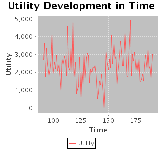
The price chart is the most important chart in the visualization
layer. It shows the development of price in each trading round (see
the section called “Price Evaluation” for details about how is this price
determined).
Current price on the
Current price on the
Y axis is displayed for
each trading round on X.
Harvest directly influences price. The importance of this chart
is to show how is price correlated with the level of current total
harvest. Some trading strategies may significantly influence price
evaluation so that the price development becomes very much independent
on current harvest level.
The quantity on the
The quantity on the
Y axis show total harvest
assigned to all traders (farmers) and the X axis
means rounds.
For each round the visualization layer draws the demand and
supply curves. Construction of those curves has been discussed in
the section called “Price Evaluation”. This chart has an overlap which the
price development chart, but it shows only the current round price
without capturing the development. It is more useful to see how
healthy the market is, how is the ability of the supply to meet demand
and also what quantity of transaction has been traded in the market in
each step.
Different trader strategies influence significantly the shape of the demand and supply curves as discussed further.
The chart shows quantity on the

Different trader strategies influence significantly the shape of the demand and supply curves as discussed further.
The chart shows quantity on the
X axis and
price on Y.

This chart show distribution of the commodity before and after
the trade round takes place. The usual pattern shows a more equal
distribution which is turned into less equally distributed commodity.
The random assignment of harvest is turned into a state where
commodity is concentrated in hands of those traders who have more
utility from each unit.
The chart displays the amount of commodity on the
The chart displays the amount of commodity on the
X axis and the amount of traders who own exactly
this amount of commodity on Y. It is basically a
distribution function. It shows how gets the commodity redistributed
after each trading round and whether there is some long-term
development in the curve shape.
The budget distribution shows where is the budget mostly
concentrated. It is divided per trader type. It shows which trader
strategy is more successful in concentrating budget. The depicted
chart is highly aggregated. It shows the number of traders for each
type who holds only units, tens, hundreds, thousands and more of
currency units.


Computerized trading is becoming more and more popular. Some of the
markets today are already mostly computer driven and trading resembles a
fight between algorithms. Algorithms may try to predict what effect do
algorithms of others have on the market and thus using this information to
better react on the development to generate bigger profit .
Computerized trading may introduce potential risks into the commodity market environment. It raises questions as for example: “What happens when most of the traders start to use computerized algorithms to trade on the market?” “Is the market still about demand and supply or is it becoming more a virtual environment which has just little to do with the commodity itself?”
Another aim of this paper is to study what happens if we introduce computerized traders into the reference model — an environment where so far only farmers with different consumer preferences traded.
Constant price fluctuations enable automatic profit generation. One of the simplest models for automatic trading is the channel breakout [3] [4] [5]. This trading strategy basically means buying at
In fact this model has many modifications and extensions, but the simplified approach above is easy to implemented into the commodity market simulation environment.
Computerized trading may introduce potential risks into the commodity market environment. It raises questions as for example: “What happens when most of the traders start to use computerized algorithms to trade on the market?” “Is the market still about demand and supply or is it becoming more a virtual environment which has just little to do with the commodity itself?”
Another aim of this paper is to study what happens if we introduce computerized traders into the reference model — an environment where so far only farmers with different consumer preferences traded.
Constant price fluctuations enable automatic profit generation. One of the simplest models for automatic trading is the channel breakout [3] [4] [5]. This trading strategy basically means buying at
n-day
minimum and selling at n-day maximum.In fact this model has many modifications and extensions, but the simplified approach above is easy to implemented into the commodity market simulation environment.
To simulate effects of computerized trading on the commodity
market a Computer Trader agent has been introduced
into the simulation environment.
The bidding strategy of the Computer Trader is completely different than for the Consumer Trader explained in the section called “The Reference Model”. Computer Traders observe the market and keep track of the maximum and minimum price for a certain number of rounds. Each round they generate buy bids for the minimum price and sell bids for the maximum. Sell bids are constrained by the available commodity units owned by the particular trader and buy bids are limited by the traders budget.
To enforce simulation heterogeneity Computer Traders as well as Consumer Traders have parameters which are set randomly within specified boundaries before simulation rounds start. One of the parameters is budget[5] and the other is number of rounds traders observe the market price to establish the minimum and maximum price used for their bidding.
Example 3. Computer trader bids
Imagine a Computer Trader with budget of
100 currency units and 5 commodity units on stock. He observers the
market price for 10 rounds and the maximum price in that period was
15 and minimum was 10. This particular agent places 5 sell bids for
15 and 10 buy bids for 10.
Bidding heterogeneity is encouraged with the number of rounds different traders observe the market which may cause different maximum and minimum prices for each trader. Imagine another trader who observers the market only for 5 rounds his maximum and minimum would be somewhere between 10 and 15. This means, Computer Trader supply will never meet another Computer trader demand. They will only be involved in transactions with Consumer Traders.
Bidding heterogeneity is encouraged with the number of rounds different traders observe the market which may cause different maximum and minimum prices for each trader. Imagine another trader who observers the market only for 5 rounds his maximum and minimum would be somewhere between 10 and 15. This means, Computer Trader supply will never meet another Computer trader demand. They will only be involved in transactions with Consumer Traders.
First we observe the market behaviour when only the
Consumer Traders are involved. Table 7, “Reference Simulation Setup” shows the parameter setting.
In the reference setup we observe significant price culminations, but it is basically a random walk around a central value, see Figure 10, “One Run of the Reference Setup” . This may be easily proven. When setting a fixed amount of harvest each turn for each trader, price gets settled on a certain number without any culminations as shown in Figure 11, “Price Development with Stable Harvest” .
The reference simulation has been run for 20 times to avoid random fluctuation. In all runs, the price starts at a quite high level (more than 25) and slowly declines each round. The closing price after 1000 rounds was in the space of 8 to 12 for the 20 runs.
The price decline is caused by the random conditions at the beginning of the simulation. During each run budged is iteratively transferred from traders who relatively prefer commodity over money to traders with reverse preferences. Every round new commodity is harvested and divided between traders. The demand and supply curve and the amount traded depends how is the commodity distributed within those two distinct groups.
This is demonstrated on the budget distribution chart where most of the traders are within the 10^3 bar (they are having thousands of currency units) when the simulation starts and as the simulation proceeds a less equal distribution is formed. Most traders are either having little budgets or on the contrary huge budgets, see Figure 10, “One Run of the Reference Setup” . The middle class slowly disappears.
Reference Simulation Setup
| Simulation | The Reference Setup |
| Rounds | 1000 |
| Budget | 1000 – 10000 |
| Harvest | 1 – 5, 10 – 40 |
| Consumer Traders | |
| Number | 30 |
| P1 | 1 – 10 |
| P2 | 50 – 200 |
In the reference setup we observe significant price culminations, but it is basically a random walk around a central value, see Figure 10, “One Run of the Reference Setup” . This may be easily proven. When setting a fixed amount of harvest each turn for each trader, price gets settled on a certain number without any culminations as shown in Figure 11, “Price Development with Stable Harvest” .


The reference simulation has been run for 20 times to avoid random fluctuation. In all runs, the price starts at a quite high level (more than 25) and slowly declines each round. The closing price after 1000 rounds was in the space of 8 to 12 for the 20 runs.
The price decline is caused by the random conditions at the beginning of the simulation. During each run budged is iteratively transferred from traders who relatively prefer commodity over money to traders with reverse preferences. Every round new commodity is harvested and divided between traders. The demand and supply curve and the amount traded depends how is the commodity distributed within those two distinct groups.
This is demonstrated on the budget distribution chart where most of the traders are within the 10^3 bar (they are having thousands of currency units) when the simulation starts and as the simulation proceeds a less equal distribution is formed. Most traders are either having little budgets or on the contrary huge budgets, see Figure 10, “One Run of the Reference Setup” . The middle class slowly disappears.

Now we are ready to simulate Computer Trader agents' influence on
the reference market model described in the section called “The Reference Setup”.
In this simulation setup, we add another 30 Computer Trader agents. They keep track of the market price for 5 - 30 rounds to determine the maximum and minimum price of their bids. Traders start trading after 150 rounds when market gets more stable.
Again the simulation has been run 20 times with this setup to avoid random fluctuation to see if some patterns of behaviour will proof to be stable.
In Figure 12, “Market Simulation Run with Computer Traders” you see a snapshot of one of the runs. It clearly demonstrates the effect of Computer Trader presence in the simulation on the price development which is significant. First the price development shows the same pattern as in the reference simulation. After round 150 Computer Trader agents start trading. The price development gets immediately affected. Its oscillation weakens each round until it gets nearly stable -/+ 1 currency unit.
Even harvest has the same characteristics as in the reference simulation, price is no more affected by the current harvest level. The presence of the new agent strategy in the market did stabilize price and made it less dependent on harvest development.
The rationale lies in the way Computer Traders react on the price development. When price is rising due to a lower total harvest level and it starts reaching agent's
Constraining price fluctuations over time causes the
Computer Trader strategy is definitely a profitable one in the reference market model. As price fluctuates the agent budget increases. But less oscillations over time means less profit for the traders.
The demand and supply curve shape is affected as well. In Figure 12, “Market Simulation Run with Computer Traders” you see large horizontal segments of the demand and supply curve. They correspond to the
The average price after 1000 rounds measured in 20 runs tend to end between 10-11 currency units which is basically the same as in the reference simulation runs. This means, the average price was not affected by the new type of trader introduced to the market but standard deviation got significantly lower.
To conclude, computerized traders did not cause any significant market failures. In fact they did stabilize the market, making price less dependent on the exogenous harvest factor.
Computerized Trader Market Setup
| Simulation | Computer Trader Market Setup |
| Rounds | 1000 |
| Budget | 1000 – 10000 |
| Harvest | 1 – 5, 10 – 40 |
| Consumer Traders | |
| Number | 30 |
| P1 | 1 – 10 |
| P2 | 50 – 200 |
| Computer Traders | |
| Number | 30 |
| Round Observed | 5 – 30 |
| Start Trading | after round 150 |
In this simulation setup, we add another 30 Computer Trader agents. They keep track of the market price for 5 - 30 rounds to determine the maximum and minimum price of their bids. Traders start trading after 150 rounds when market gets more stable.
Again the simulation has been run 20 times with this setup to avoid random fluctuation to see if some patterns of behaviour will proof to be stable.
In Figure 12, “Market Simulation Run with Computer Traders” you see a snapshot of one of the runs. It clearly demonstrates the effect of Computer Trader presence in the simulation on the price development which is significant. First the price development shows the same pattern as in the reference simulation. After round 150 Computer Trader agents start trading. The price development gets immediately affected. Its oscillation weakens each round until it gets nearly stable -/+ 1 currency unit.

Even harvest has the same characteristics as in the reference simulation, price is no more affected by the current harvest level. The presence of the new agent strategy in the market did stabilize price and made it less dependent on harvest development.
The rationale lies in the way Computer Traders react on the price development. When price is rising due to a lower total harvest level and it starts reaching agent's
n-round maximum they react by selling their stock
commodities. This brings more commodity to the market causing price to
fall. Analogically, higher harvest causing the price to fall reaching
agents' minimum price makes agents buy and thus turning the fall into
growth again.Constraining price fluctuations over time causes the
n-round maximum and minimum to shrink. This makes the
agents buy and sell earlier when price fluctuates and thus shrinking the
price oscillation more and more until is gets bounded on a certain
price.Computer Trader strategy is definitely a profitable one in the reference market model. As price fluctuates the agent budget increases. But less oscillations over time means less profit for the traders.
The demand and supply curve shape is affected as well. In Figure 12, “Market Simulation Run with Computer Traders” you see large horizontal segments of the demand and supply curve. They correspond to the
n-round maximum (supply) and minimum (demand) prices
the agents did establish. This horizontal segments start to emerge after
the 150th round. First there is a significant
gap between both curves but it shrinks with each round as the agents'
n-round maximum comes closer to the minimum.The average price after 1000 rounds measured in 20 runs tend to end between 10-11 currency units which is basically the same as in the reference simulation runs. This means, the average price was not affected by the new type of trader introduced to the market but standard deviation got significantly lower.
To conclude, computerized traders did not cause any significant market failures. In fact they did stabilize the market, making price less dependent on the exogenous harvest factor.
One of the popular aims of automated market simulations is to
simulate different market failures. For example [2]
simulates market price bubbles using near zero-intelligent agents.
Market bubbles do not occur with rational traders. From various studies [1] [2] it seams bubbles are related to some kind of cognitive failures of traders. Zero-intelligent agents are basically traders who act nearly randomly. It simulates real life traders with minimum background knowledge who do not act rationally and their behaviour resembles random decisions.
This paper focuses on another frequently mentioned reason for market bubbles which is groupthink and herd behavior. Yet another trading strategy has been introduced into the simulation described in this paper — the Trend Trader.
In contrast to zero-intelligent agents, the Trend
Trader agent is a representative of a trading strategy which
actually makes sense in some situations. This type of agent expects the
market to follow certain stable trends. In case price is a random walk
this trader is going to loose money over time. But in case there is a
significant trend factor in the price development, this trader may be
involved in profitable transactions.
The Trend Trader keeps a history of prices and calculates a trend out of it. According to the trend he predicts the price in the following round. In case the trend is positive the agent places buy bids on the market as he expects the trend to continue. In case trend is negative the agent sells.
This strategy is closely related to groupthink or herd behaviour as agents simply expect others to behave similarly which will cause the trend to continue. In case there is a positive price trend the prospects are positive and everyone is buying, the agent predicts the price to continue to rise. He is buying, as he expects he can sell for even more later. As soon as the trend changes, the agent expects the market just passed a peak and he starts selling while price is still high.
Analogically to Computer Traders, Trend Traders observe market price for a certain period (one of the parameters) and each turn they calculate trend out of the recent price history. Expected price Pe is calculated as an the current price
Trend

The Trend Trader keeps a history of prices and calculates a trend out of it. According to the trend he predicts the price in the following round. In case the trend is positive the agent places buy bids on the market as he expects the trend to continue. In case trend is negative the agent sells.
This strategy is closely related to groupthink or herd behaviour as agents simply expect others to behave similarly which will cause the trend to continue. In case there is a positive price trend the prospects are positive and everyone is buying, the agent predicts the price to continue to rise. He is buying, as he expects he can sell for even more later. As soon as the trend changes, the agent expects the market just passed a peak and he starts selling while price is still high.
Analogically to Computer Traders, Trend Traders observe market price for a certain period (one of the parameters) and each turn they calculate trend out of the recent price history. Expected price Pe is calculated as an the current price
P and the
n-round trend
Tn.Trend
Tn is calculated
as average ΔP for rounds r -
n .. r - 1, where
r is the current round number[6].
Example 4. Trend Trader Bidding
Image a Trend Trader who observers the
price market for
Tn = 20 / 5 = 4, expected price in round 206 is 44 currency units. Trend is positive, the trader expects price to increase and thus he is buying.
n = 6 rounds. He has a budget of
150 currency units and 5 commodity units on stock.
Observed Price History
Round r | 200 | 201 | 202 | 203 | 204 | 205 | 206 |
Price P | 20 | 25 | 34 | 36 | 30 | 40 | - |
ΔP | - | 5 | 9 | 2 | -6 | 10 | - |
| Trend | 20 | 24 | 28 | 32 | 36 | 40 | 44 |
| ΔTrend | 4 | 4 | 4 | 4 | 4 | 4 |
Tn = 20 / 5 = 4, expected price in round 206 is 44 currency units. Trend is positive, the trader expects price to increase and thus he is buying.
 |

In the next simulation series we place Consumer Traders
together with Trend Traders in the
commodity market.
As discussed earlier, price development in the solely Consumer Trader market is basically a random walk correlated with harvest which is a random function. There are no trends for a purely random variable, there is just noise. This causes Trend Traders to mistakenly recognize trends where there are non.
As a result Trend Traders really cause short-term bubbles to occur on the market, but they are incrementally loosing money on them. As their budget decreases, their ability to place bids lowers until the market starts behaving as if no other agents than Consumer Traders where present on the market.
Figure 13, “Simulation Run with Consumer and Trend Traders” demonstrates the behaviour explained above on a simulation snapshot. Even harvest is a random walk, price development depicts significant bubbles. The price starts dramatically rising reaching its peak in circa 20 - 30 rounds. Than it falls straight down again in less than 10 rounds. The budget distribution chart already shows Trend Traders starting to loose their budgets. The most frequent category has only 10s of currency units so they are unable to influence the market significantly.
As Trend Traders loose money, bubbles tend to weaken until finally the price returns into a random walk correlated only with the harvest. The supply curve shape is significantly influenced by the agent behavior. As trend is currently negative in the snapshot, most Trend Traders bid to sell for a similar quite low price.
During the upward trend agents start buying and thus reversely the demand curve shape is affected showing a large horizontal segment as seen in Figure 14, “Upward Trend”. In the same figure we see how is price development turned from a random walk into bubbles as soon as Trend Traders start to trade (after round 150).
Figure 15, “Back to Random Walk” depicts how is the “bubbled” price development incrementally turned back to random noise. The budget distribution chart shows the majority of Trend Traders having just 10s of currency units so they do not affect price evaluation anymore.
The presence of Trend Traders affects average price during simulation runs. Even finally average price in 20 runs turns to be 12 which is similar to the previous setups, it is probably because of the relatively short period Trend Traders have to affect the market. During the time Trend Traders are active on the market, average price gets up to 30 currency units.
Trend Traders with Consumer Traders Simulation Setup
| Simulation | Trend and Consumer Trader Setup |
| Rounds | 1000 |
| Budget | 1000 – 10000 |
| Harvest | 1 – 5, 10 – 40 |
| Consumer Traders | |
| Number | 30 |
| P1 | 1 – 10 |
| P2 | 50 – 200 |
| Trend Traders | |
| Number | 30 |
| Round Observed | 5 – 30 |
| Start Trading | after round 150 |
As discussed earlier, price development in the solely Consumer Trader market is basically a random walk correlated with harvest which is a random function. There are no trends for a purely random variable, there is just noise. This causes Trend Traders to mistakenly recognize trends where there are non.
As a result Trend Traders really cause short-term bubbles to occur on the market, but they are incrementally loosing money on them. As their budget decreases, their ability to place bids lowers until the market starts behaving as if no other agents than Consumer Traders where present on the market.
Figure 13, “Simulation Run with Consumer and Trend Traders” demonstrates the behaviour explained above on a simulation snapshot. Even harvest is a random walk, price development depicts significant bubbles. The price starts dramatically rising reaching its peak in circa 20 - 30 rounds. Than it falls straight down again in less than 10 rounds. The budget distribution chart already shows Trend Traders starting to loose their budgets. The most frequent category has only 10s of currency units so they are unable to influence the market significantly.
As Trend Traders loose money, bubbles tend to weaken until finally the price returns into a random walk correlated only with the harvest. The supply curve shape is significantly influenced by the agent behavior. As trend is currently negative in the snapshot, most Trend Traders bid to sell for a similar quite low price.
During the upward trend agents start buying and thus reversely the demand curve shape is affected showing a large horizontal segment as seen in Figure 14, “Upward Trend”. In the same figure we see how is price development turned from a random walk into bubbles as soon as Trend Traders start to trade (after round 150).

Figure 15, “Back to Random Walk” depicts how is the “bubbled” price development incrementally turned back to random noise. The budget distribution chart shows the majority of Trend Traders having just 10s of currency units so they do not affect price evaluation anymore.

The presence of Trend Traders affects average price during simulation runs. Even finally average price in 20 runs turns to be 12 which is similar to the previous setups, it is probably because of the relatively short period Trend Traders have to affect the market. During the time Trend Traders are active on the market, average price gets up to 30 currency units.

The highpoint of this paper is the following setup where all
trader types are put together into the same simulation
environment.
With all three trader types involved the simulation becomes complex and difficult to interpret. Testing experiences have shown with all trader types together even a very little change in the behaviour of one trader could be multiplied in combination with some features of other agent types causing unpredicted results.
Figure 16, “Simulation Run Snapshot — All Traders” depicts one of simulation run snapshots. The price development shows very interesting patterns. Price is extremely unstable in a longer run but showing segments of stability for shorter time periods. It seems as if Computer Traders would compete with Trend Traders over who is causes the major influence on price and some developments are more favourable to either the first or the second group.
An important discovery conducted from this simulation setup is: Trend Traders actually become profitable if accompanied with Computer Traders on the market. The budget distribution chart shows many Trend Traders still with budget of 1000s currency units even the round did already pass 450. This is a stable phenomenon observer in many different runs with this setup.
The cause may likely be explained by the Computer Trader's effect on price reducing random walk which is harmful for Trend Traders. Shifts between periods where price is mostly influence by one or the other trader group may be explained by budget fluctuations between trader groups.
Imagine Trend Traders rule the market and a steep price increase has just begun. More and more traders start to realize a positive trend and they buy causing the price to rise even more. After a while Trend Traders consume most of their budget for commodity, less buy bids are issued and price increase starts to slow down. This continues until the peak is met and Trend Traders loose their ability to cause further increase.

At this time, price reaches ridiculous proportions with no relation to harvest which is the only price maker in the reference model. As a result, price starts to fall down quickly to it reference model natural average around the value of 10. Trend Traders who first notice the trend[7] shift have opportunity to earn as they start selling at high prices, others will loose because of the bubble. At this point Trend Traders start to cumulate budget again and they are accelerating the price fall.
Bubbles are less advantageous for Computer Traders who benefit especially in the random walk environment. They were selling to the Trend Traders during the price increase in the first phase of the bubble. Now when price decreases they wait until it reaches their
As price falls more and more, traders reach their minimums and they start buying. They cumulated budget during the rise phase so they are strong enough to stop the fall for few rounds. This creates the distinctive horizontal segments in the price curve.
It is important to note that the partial explanations above are only speculations. There is no evidence that the price development was really significantly influenced by the mentioned causes. The simulation already reached the point where it mostly resembles a black box and deeper understanding of the model would require better diagnostic tools and much deeper insight.
In 20 runs the average price during this simulation setup was stable around 18 currency units which is nearly the double of the average price measured in the reference model.
Different price bubbles are very frequent during this simulation setup as demonstrated by Figure 17, “Captured Price Bubble Gallery”. They basically appear constantly during the whole run. No trader groups tends to get out of budget during simulations.

Simulation Setup with All Agent Types
| Simulation | Consumer, Computer and Trend Traders |
| Rounds | 1000 |
| Budget | 1000 – 10000 |
| Harvest | 1 – 5, 10 – 40 |
| Consumer Traders | |
| Number | 30 |
| P1 | 1 – 10 |
| P2 | 50 – 200 |
| Computer Traders | |
| Number | 30 |
| Round Observed | 5 – 30 |
| Trend Traders | |
| Number | 30 |
| Round Observed | 5 – 30 |
With all three trader types involved the simulation becomes complex and difficult to interpret. Testing experiences have shown with all trader types together even a very little change in the behaviour of one trader could be multiplied in combination with some features of other agent types causing unpredicted results.
Figure 16, “Simulation Run Snapshot — All Traders” depicts one of simulation run snapshots. The price development shows very interesting patterns. Price is extremely unstable in a longer run but showing segments of stability for shorter time periods. It seems as if Computer Traders would compete with Trend Traders over who is causes the major influence on price and some developments are more favourable to either the first or the second group.
An important discovery conducted from this simulation setup is: Trend Traders actually become profitable if accompanied with Computer Traders on the market. The budget distribution chart shows many Trend Traders still with budget of 1000s currency units even the round did already pass 450. This is a stable phenomenon observer in many different runs with this setup.
The cause may likely be explained by the Computer Trader's effect on price reducing random walk which is harmful for Trend Traders. Shifts between periods where price is mostly influence by one or the other trader group may be explained by budget fluctuations between trader groups.
Imagine Trend Traders rule the market and a steep price increase has just begun. More and more traders start to realize a positive trend and they buy causing the price to rise even more. After a while Trend Traders consume most of their budget for commodity, less buy bids are issued and price increase starts to slow down. This continues until the peak is met and Trend Traders loose their ability to cause further increase.


At this time, price reaches ridiculous proportions with no relation to harvest which is the only price maker in the reference model. As a result, price starts to fall down quickly to it reference model natural average around the value of 10. Trend Traders who first notice the trend[7] shift have opportunity to earn as they start selling at high prices, others will loose because of the bubble. At this point Trend Traders start to cumulate budget again and they are accelerating the price fall.
Bubbles are less advantageous for Computer Traders who benefit especially in the random walk environment. They were selling to the Trend Traders during the price increase in the first phase of the bubble. Now when price decreases they wait until it reaches their
n-round minimum. Those
with higher n are better off as they start buying
later for less. The Computer Trader's behaviour is
likely responsible for the stair-like effect during the price fall
phase.As price falls more and more, traders reach their minimums and they start buying. They cumulated budget during the rise phase so they are strong enough to stop the fall for few rounds. This creates the distinctive horizontal segments in the price curve.
It is important to note that the partial explanations above are only speculations. There is no evidence that the price development was really significantly influenced by the mentioned causes. The simulation already reached the point where it mostly resembles a black box and deeper understanding of the model would require better diagnostic tools and much deeper insight.
In 20 runs the average price during this simulation setup was stable around 18 currency units which is nearly the double of the average price measured in the reference model.
Different price bubbles are very frequent during this simulation setup as demonstrated by Figure 17, “Captured Price Bubble Gallery”. They basically appear constantly during the whole run. No trader groups tends to get out of budget during simulations.


This paper demonstrates how to build an automated simulation
environment from scratch and how to simulate complex real life patterns
which are very difficult to be studied analytically.
Complexity has been introduced iteratively. First, each trader strategy has been studied separately causing predictable and clearly explainable results. After all three very simple trader strategies described in this paper were put together into the same simulation setup, very complex patterns emerged.
This demonstrates a synergic effect known from the system theory. Adding few simple elements into the system influencing each other is causing complex results which are difficult to predict or analyze.
There are also other consequences of the observed simulation runs. The commodity market has it's moral dimension as availability of the commodities traded on the market are essential for people's basic survival. Different simulation setups allowed as to study the influence of different trading strategies on the reference model which is composed solely of traders who are in fact also consumers of the commodity.
This paper has shown that some trading strategies may be neutral or even beneficial for the consumers, but other may cause unpredictable developments and price bubbles which are very dangerous especially on the commodity market for reasons mentioned in the section called “Commodity Market”.
Simulation involving the computerized traders made the market less vulnerable to seasonal influences[9], which was beneficial to consumers as it gave them a stable environment with price less dependent on random factors. At the same time, the long term average price was nearly the same as in the reference model.
On the other hand, the final simulation setup with all three trader types involved has shown an hostile environment for the consumers. Trend Traders cause price bubble which increases price for regular consumers up to 700% during peaks and Computer Traders preserve them so bubbles last longer. Bubbles even longer than 100 rounds has been observed during different simulation runs.
The average price during the 1000 simulation rounds has shown to be double of the average price in the reference model.
A. Implementation
The simulation environment described in the previous sections has been implemented from scratch by the author of this paper. No simulation framework has been used. The whole system has rather been implemented specifically in Java programming language using a specific object model, see Figure A.1, “The Simulation High-level Object Model”.JFreeChart library for rendering different chart types has been used for the visualization layer which is basically a Swing application.
The main
Simulation class is the place where
to setup different parameters of the simulation run. Each round is
calculated in Market which holds collections of
traders. Buy and sell Bids are collected for each
trader, ordered ascending and descending to form the demand and supply
series. After equilibrium price is determined the market is cleared and
transactions between traders are processed.Each round during calculation the
Market
notifies all registered IMarketListeners about
development in commodity, budget, price, demand, supply and utility. There
is just one implemented listener which is the
Dashboard. It is a Swing
JFrame and it contains all the charts described in
the section called “Visualization”. Some charts are updated before
the round starts[10] and all are updated after the round finishes.Any trader who implements the
ITrader
interface may be easily plugged to participate in the simulation. If the
trader extends the AbstractTrader class, it only
needs to implement the following methods:
getBuyBids(),
getSellBids(),
priceUpdate(),
consumeCommodity(). The different trading
strategies (Consumer Trader, Trend
Trader and Computer Trader) differ only in
the implementation of those 4 methods.The abstract class executes all the functionality the agents have in common, for example updating the commodity variable in can agents did buy some or updating the budget in case transactions are made etc...


To demonstrate how easy it is to bring a new trader into the simulation, lets assume we intend to introduce a Random Trader who acts randomly ignoring price signals from the market. Example A.1, “Random Trader Implementation” shows the implementation code[11].
Example A.1. Random Trader
Implementation
public class RandomTrader extends AbstractTrader {

    public RandomTrader(long budget, long commodity) {
        this.budget = budget;
        this.commodity = commodity;
    }

    public Collection<IBid> getBuyingBids() {
        Collection<IBid> bids = new ArrayList<IBid>();
        long totalPriceBid = 0;
        while (totalPriceBid < budget) {
            long bidPrice = getRandomPrice();
            totalPriceBid = totalPriceBid + bidPrice;
            bids.add(new Bid(this, bidPrice));
        }
        return bids;
    }

    public Collection<IBid> getSellingBids() {
        Collection<IBid> bids = new ArrayList<IBid>();
        for (int i = 0; i < commodity; i++) {
            bids.add(new Bid(this, getRandomPrice()));
        }
        return bids;
    }


    public void priceInfo(long price) {
        // ignore
    }

    public void consumeAll() {
        //ignore
    }

}
[1] Gil-bazo, J., Moreno, D., Tapia,
M.:Price dynamics, informational efficiency, and wealth
distribution in continuous double-auction markets. Universidad
Carlos III. Spain. 2007.
[2] Duffy, J., Unver, U.:Asset price
bubbles and crashes with near-zero-intelligence traders. Economic
Theory Journal. Berlin. 2005. ISSN 0938-2259
[4] Mayers, D.:Applying The Noise
Channel System to IBM 5min Bars. Futures. Chicago. 2001.
URL: http://www.meyersanalytics.com/papers.php
[5] Katz, J., McCormick,
D.:Encyclopedia of Trading Strategies. McGraw-Hill. 2000.
ISBN: 00-70580-99-5
[1] Raw agricultural commodities traded on the commodity markets
include corn, oats, rough rice, soybeans, soybean meal, soybean oil.
wheat, cocoa, coffee, cotton, sugar.
[2] The average value is ( min + max / 2 ) multiplied by the
number of farmers involved.
[3] Obviously each unit is bid for a different sell price. With a
diminishing marginal utility function, the last unit is the cheapest
and every previous unit is offered for more. Similarly when buying
units, one unit would be bought for less than the next unit.
[4] Another obvious limit for bids: price needs to stay
positive.
[5] This is the very same budget parameter used to setup initial
budgets for Consumer Traders.
[6] Of course more sophisticated statistical methods may be used
as for example regression or interpolation but this simple method
does its job just fine for the simulation objectives.
[8] Note the Prague Castle-like shape of many of the simulated
price bubbles.
[9] They did smoothen the harvest fluctuation and their effect on
price.
[10] For example the commodity distribution chart shows distribution
before trading starts (after harvest) and how did the distribution
change because of trading.
[11] To simplify the code, the
getRandomPrice() method has not been
implemented in the example.